· Python · 12 min read
Learn geopandas by plotting tornados on a map
In this tutorial we will take a look at the powerful geopandas library and use it to plot historical tornado data on a map of the United States. We will use two different shapefiles from NOAA, the...
This post was originally published on jcutrer.com (WordPress) and has been migrated to the archive.
In this tutorial we will take a look at the powerful geopandas library and use it to plot historical tornado data on a map of the United States.
We will use two different shapefiles from NOAA, the first dataset includes the origination point for each tornado. The second dataset includes a line path of each tornado. The data comes from the NOAA Storm Prediction Center an can be downloaded from (https://www.spc.noaa.gov/gis/svrgis/)
A quick note before we start
I assume you know some basic python and how to install jupyter to run the companion notebook. To get started, clone my git repository with the following commands.
git clone https://github.com/joncutrer/geopandas-tutorial
cd geopandas-tutorial
jupyter notebook
Here are the commands you will need to run if have not already install geopandas.
conda install geopandas
conda install -c conda-forge descartes
The data we will be working with comes from the US Census and is in a common shapefile format.
ls -al datatotal 11044
drwxrwxr-x 2 sysadmin sysadmin 4096 May 3 19:45 ./
drwxrwxr-x 5 sysadmin sysadmin 4096 May 6 23:11 ../
-rw-rw-r-- 1 sysadmin sysadmin 3929143 Oct 1 2019 1950-2018-torn-aspath.zip
-rw-rw-r-- 1 sysadmin sysadmin 3191635 Oct 1 2019 1950-2018-torn-initpoint.zip
-rw-rw-r-- 1 sysadmin sysadmin 3808548 May 2 2019 cb_2018_48_tract_500k.zip
-rw-rw-r-- 1 sysadmin sysadmin 5 May 1 20:37 usa-states-census-2014.cpg
-rw-rw-r-- 1 sysadmin sysadmin 15201 May 1 20:37 usa-states-census-2014.dbf
-rw-rw-r-- 1 sysadmin sysadmin 143 May 1 20:37 usa-states-census-2014.prj
-rw-rw-r-- 1 sysadmin sysadmin 257 May 1 20:37 usa-states-census-2014.qpj
-rw-rw-r-- 1 sysadmin sysadmin 309672 May 1 20:37 usa-states-census-2014.shp
-rw-rw-r-- 1 sysadmin sysadmin 18517 May 1 20:37 usa-states-census-2014.shp.xml
-rw-rw-r-- 1 sysadmin sysadmin 564 May 1 20:37 usa-states-census-2014.shxImport geopandas and load the U.S. map shapefile
import matplotlib.pyplot as plt
import geopandas
states = geopandas.read_file('data/usa-states-census-2014.shp')
states.head() STATEFP
STATENS
AFFGEOID
GEOID
STUSPS
NAME
LSAD
ALAND
AWATER
region
geometry
0
06
01779778
0400000US06
06
CA
California
00
403483823181
20483271881
West
MULTIPOLYGON Z (((-118.59397 33.46720 0.00000,...
1
11
01702382
0400000US11
11
DC
District of Columbia
00
158350578
18633500
Northeast
POLYGON Z ((-77.11976 38.93434 0.00000, -77.04...
2
12
00294478
0400000US12
12
FL
Florida
00
138903200855
31407883551
Southeast
MULTIPOLYGON Z (((-81.81169 24.56874 0.00000, ...
3
13
01705317
0400000US13
13
GA
Georgia
00
148963503399
4947080103
Southeast
POLYGON Z ((-85.60516 34.98468 0.00000, -85.47...
4
16
01779783
0400000US16
16
ID
Idaho
00
214045425549
2397728105
West
POLYGON Z ((-117.24303 44.39097 0.00000, -117....Reproject coordinates
By default this shp file is in WGS 84.
states.crs
Name: WGS 84
Axis Info :
- Lat: Geodetic latitude (degree)
- Lon: Geodetic longitude (degree)
Area of Use:
- name: World
- bounds: (-180.0, -90.0, 180.0, 90.0)
Datum: World Geodetic System 1984
- Ellipsoid: WGS 84
- Prime Meridian: Greenwich
To make the map look a little more familiar lets reproject it’s coordinates to Mercator.
states = states.to_crs("EPSG:3395")Now lets plot the U.S. map and see what we get
states.plot()!(/wp-content/uploads/2020/05/6-united-states-plot.png)
We can also plot the state polygons with no fill color by using boundary.
states.boundary.plot()!(/wp-content/uploads/2020/05/7-united-states-plot.png)
Load the NOAA US tornado dataset
Source: (https://www.spc.noaa.gov/gis/svrgis/)
One of the cool features of geopandas is that you can load a shapefile directly from a zip archive without first unzipping it. The file path to open a zipped shapefile is prefixed with zip://
However, there is a caveat. If the zip archive contains a subfolder you must specify it by appending !foldername to the path.
ls -al datatotal 11044
drwxrwxr-x 2 sysadmin sysadmin 4096 May 3 19:45 ./
drwxrwxr-x 5 sysadmin sysadmin 4096 May 6 23:11 ../
-rw-rw-r-- 1 sysadmin sysadmin 3929143 Oct 1 2019 1950-2018-torn-aspath.zip
-rw-rw-r-- 1 sysadmin sysadmin 3191635 Oct 1 2019 1950-2018-torn-initpoint.zip
-rw-rw-r-- 1 sysadmin sysadmin 3808548 May 2 2019 cb_2018_48_tract_500k.zip
-rw-rw-r-- 1 sysadmin sysadmin 5 May 1 20:37 usa-states-census-2014.cpg
-rw-rw-r-- 1 sysadmin sysadmin 15201 May 1 20:37 usa-states-census-2014.dbf
-rw-rw-r-- 1 sysadmin sysadmin 143 May 1 20:37 usa-states-census-2014.prj
-rw-rw-r-- 1 sysadmin sysadmin 257 May 1 20:37 usa-states-census-2014.qpj
-rw-rw-r-- 1 sysadmin sysadmin 309672 May 1 20:37 usa-states-census-2014.shp
-rw-rw-r-- 1 sysadmin sysadmin 18517 May 1 20:37 usa-states-census-2014.shp.xml
-rw-rw-r-- 1 sysadmin sysadmin 564 May 1 20:37 usa-states-census-2014.shxLoad the shapefile from zip archive
We will use the above mentioned technique to load the 1950-2018-torn-initpoint.shp shapefile from the zip archive.
tornados = geopandas.read_file(
    'zip://data/1950-2018-torn-initpoint.zip!1950-2018-torn-initpoint'
)
Note: If loading from inside a zip file confuses you don’t let is slow you down, just unzip the archive.
Lets have a look at the DataFrame
tornados.shape(63645, 23)tornados.info()
RangeIndex: 63645 entries, 0 to 63644
Data columns (total 23 columns):
 #   Column    Non-Null Count  Dtype
---  ------    --------------  -----
 0   om        63645 non-null  int64
 1   yr        63645 non-null  int64
 2   mo        63645 non-null  int64
 3   dy        63645 non-null  int64
 4   date      63645 non-null  object
 5   time      63645 non-null  object
 6   tz        63645 non-null  int64
 7   st        63645 non-null  object
 8   stf       63645 non-null  int64
 9   stn       63645 non-null  int64
 10  mag       63645 non-null  int64
 11  inj       63645 non-null  int64
 12  fat       63645 non-null  int64
 13  loss      63645 non-null  float64
 14  closs     63645 non-null  float64
 15  slat      63645 non-null  float64
 16  slon      63645 non-null  float64
 17  elat      63645 non-null  float64
 18  elon      63645 non-null  float64
 19  len       63645 non-null  float64
 20  wid       63645 non-null  int64
 21  fc        63645 non-null  int64
 22  geometry  63645 non-null  geometry
dtypes: float64(7), geometry(1), int64(12), object(3)
memory usage: 11.2+ MB
tornados om
yr
mo
dy
date
time
tz
st
stf
stn
...
loss
closs
slat
slon
elat
elon
len
wid
fc
geometry
0
1
1950
1
3
1950-01-03
11:00:00
3
MO
29
1
...
6.0
0.0
38.7700
-90.2200
38.8300
-90.0300
9.50
150
0
POINT (-90.22000 38.77000)
1
2
1950
1
3
1950-01-03
11:55:00
3
IL
17
2
...
5.0
0.0
39.1000
-89.3000
39.1200
-89.2300
3.60
130
0
POINT (-89.30000 39.10000)
2
3
1950
1
3
1950-01-03
16:00:00
3
OH
39
1
...
4.0
0.0
40.8800
-84.5800
40.8801
-84.5799
0.10
10
0
POINT (-84.58000 40.88000)
3
4
1950
1
13
1950-01-13
05:25:00
3
AR
5
1
...
3.0
0.0
34.4000
-94.3700
34.4001
-94.3699
0.60
17
0
POINT (-94.37000 34.40000)
4
5
1950
1
25
1950-01-25
19:30:00
3
MO
29
2
...
5.0
0.0
37.6000
-90.6800
37.6300
-90.6500
2.30
300
0
POINT (-90.68000 37.60000)
...
...
...
...
...
...
...
...
...
...
...
...
...
...
...
...
...
...
...
...
...
...
63640
617020
2018
12
27
2018-12-27
10:15:00
3
LA
22
0
...
7000.0
0.0
30.1302
-92.3645
30.1321
-92.3547
0.60
25
0
POINT (-92.36450 30.13020)
63641
617021
2018
12
27
2018-12-27
10:29:00
3
MS
28
0
...
15000.0
0.0
32.6431
-90.4509
32.6427
-90.4288
1.29
100
0
POINT (-90.45090 32.64310)
63642
617022
2018
12
31
2018-12-31
12:35:00
3
KY
21
0
...
55000.0
0.0
36.8900
-87.9870
36.8915
-87.9734
0.76
125
0
POINT (-87.98700 36.89000)
63643
617023
2018
12
31
2018-12-31
13:43:00
3
IN
18
0
...
50000.0
0.0
38.1813
-86.8863
38.2006
-86.8585
2.01
50
0
POINT (-86.88630 38.18130)
63644
617024
2018
12
31
2018-12-31
14:38:00
3
IN
18
0
...
20000.0
0.0
38.0935
-86.0869
38.1000
-86.0470
2.20
140
0
POINT (-86.08690 38.09350)63645 rows × 23 columns
Reproject coordinates
We will also need to reproject it’s coordinates to Mercator so that our maps line up.
tornados = tornados.to_crs("EPSG:3395")Take note how reprojecting our coordinates to Mercator moves the decimal point in our lat, long data. This will come into play later.
tornados[:1].geometry0 POINT (-10043244.459 4662018.860)
Name: geometry, dtype: geometryOur first plot of U.S. tornado data
tornados.plot( figsize=(12,9), color='red', marker='x', markersize=1)!(/wp-content/uploads/2020/05/15-tornados-plot.png)
Now lets plot the tornados data on top of the U.S. basemap
import matplotlib.pyplot as plt
fig = plt.figure(1, figsize=(12,9))
ax = fig.add_subplot()
states.boundary.plot(ax=ax, color='black', linewidth=.8)

tornados.plot(ax=ax, color='red', marker='.', markersize=1)
!(/wp-content/uploads/2020/05/16-tornados-plot.png)
Wow, that’s great!
We even chose an ominous red v-shaped marker to represent the tornados. The two maps line up perfectly but it looks like we have some outliers data for Hawaii, Alaska, and Puerto Rico that are stretching out our map canvas.
We want to focus on the lower 48 states so now we need to narrow down our view. We can accomplish this in a couple of ways. One way is to remove any tornados from our dataframe that are not in the lower 48. Another approach is to simply limit the viewport area of the map with ax.set_xlim() and ax.set_ylim().
Our first thought might be to pass in typical lat,long data such as ax.set_xlim(-101.12345, 72.12345). After we reprojected our maps to Mercator our coordinates data now looks like this ax.set_xlim(-10112345, 7212345).
import matplotlib.pyplot as plt
fig = plt.figure(1, figsize=(12,9))
ax = fig.add_subplot()

# US Lower 48 Bounding Box
# -141.00000, 26.00000, -65.50000, 72.00000

ax.set_xlim(-14100244, -7200000)
ax.set_ylim(2600000, 6550000)

fig.suptitle('United States Tornado Map (1950-2018)', fontsize=16)

states.boundary.plot(ax=ax, color='black', linewidth=.8)

tornados.plot(ax=ax, color='red', marker='v', markersize=8)
!(/wp-content/uploads/2020/05/17-tornados-plot.png)
Hey! That was a success, now let’s press on.
Get total tornados by State
I already know the answer to this question (because its my home) but… Which state do you think has had the most tornados?
Hint: In Texas we call them twisters
# Create a copy of the original DataFrame
twisters_by_state = tornados.copy()
# Add a new column and set the value to 1
twisters_by_state['tornados'] = 1

# use groupby() and count() to total up all the tornadoes by state
twisters_by_state = twisters_by_state[['st','tornados']].groupby('st').count()

# sort by most tornadoes first
twisters_by_state.sort_values('tornados', ascending=False).head(10)
Yep, Texas has the most tornados!
We can also easily plot this data by calling plot()
twisters_by_state.plot.bar(figsize=(12,6), title='Tornados by State (1950-2018)')!(/wp-content/uploads/2020/05/19-tornados-by-state.png)
Notice that our sorting did not stick, this is because we did not reassign the DataFrame only output it to the screen.
We can chain in a call to .sort_values() to get our ordering to work in the plot.
I will also select the top 10 be adding [:10] which means “slice first 10 rows”.
Now we can see our state labels a little better.
twisters_by_state.sort_values('tornados', ascending=False)[:10].plot.bar(figsize=(12,6), title='Tornados by State (Top 10)')!(/wp-content/uploads/2020/05/20-tornados-by-state-top10.png)
If we just want a list of the top 10 states we can do something like this.
top10 = twisters_by_state.sort_values('tornados', ascending=False)[:10].index
top10
Index(['TX', 'KS', 'OK', 'FL', 'NE', 'IA', 'IL', 'MO', 'MS', 'CO'], dtype='object', name='st')Plot tornados by state
Now that we know that Texas has had the most tornados lets subset our tornado dataset to only show Texas Twisters.
texas_map = states == 'Texas']
texas_map.plot()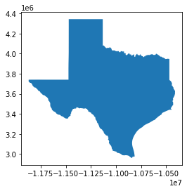
texas_twisters = tornados == 'TX']
texas_twisters
om
yr
mo
dy
date
time
tz
st
stf
stn
...
loss
closs
slat
slon
elat
elon
len
wid
fc
geometry
6
7
1950
1
26
1950-01-26
18:00:00
3
TX
48
1
...
0.0
0.0
26.8800
-98.1200
26.8800
-98.0500
4.70
133
0
POINT (-10922668.437 3089173.889)
7
8
1950
2
11
1950-02-11
13:10:00
3
TX
48
2
...
4.0
0.0
29.4200
-95.2500
29.5200
-95.1300
9.90
400
0
POINT (-10603181.498 3408227.270)
...
...
...
...
...
...
...
...
...
...
...
...
...
...
...
...
...
...
...
...
...
...
63637
617017
2018
12
26
2018-12-26
15:40:00
3
TX
48
0
...
30000.0
0.0
33.7772
-100.7792
33.7819
-100.7780
0.34
30
0
POINT (-11218689.227 3975169.719)
63638
617018
2018
12
26
2018-12-26
16:23:00
3
TX
48
0
...
0.0
0.0
34.9310
-100.8941
34.9342
-100.8849
0.57
100
0
POINT (-11231479.836 4130042.118)8804 rows × 23 columns
texas_twisters.plot(markersize=1)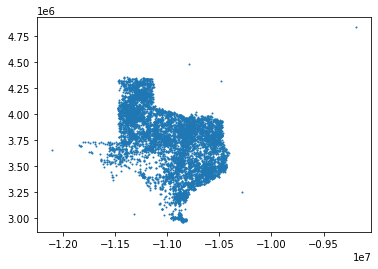
Now that we have both of our DataFrames texas_map and texas_twisters lets overlay combine and plot them.
import matplotlib.pyplot as plt
fig = plt.figure(1, figsize=(10,10))
ax = fig.add_subplot()

# Adjust bounding box to only Texas
# -119.00000, 29.30000, -103.80000, 44.00000

ax.set_xlim(-11910000, -10380000)
ax.set_ylim(2930000, 4400000)

fig.suptitle('Texas Tornados (1950-2018)', fontsize=16)

texas_map.boundary.plot(ax=ax, color='black', linewidth=.8)

texas_twisters.plot(ax=ax, color='red', marker='v', markersize=20)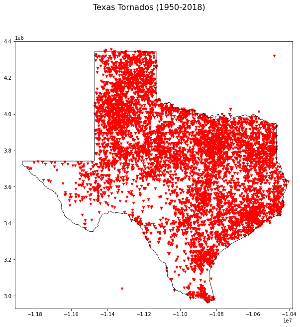
Now lets move over to the path shapefile and see what we have to work with.
Load the NOAA US tornado paths dataset
tornado_paths = geopandas.read_file('zip://data/1950-2018-torn-aspath.zip!1950-2018-torn-aspath')tornado_paths.head() om
yr
mo
dy
date
time
tz
st
stf
stn
...
loss
closs
slat
slon
elat
elon
len
wid
fc
geometry
0
1
1950
1
3
1950-01-03
11:00:00
3
MO
29
1
...
6.0
0.0
38.77
-90.22
38.8300
-90.0300
9.5
150
0
LINESTRING (-90.22000 38.77000, -90.03000 38.8...
1
2
1950
1
3
1950-01-03
11:55:00
3
IL
17
2
...
5.0
0.0
39.10
-89.30
39.1200
-89.2300
3.6
130
0
LINESTRING (-89.30000 39.10000, -89.23000 39.1...
2
3
1950
1
3
1950-01-03
16:00:00
3
OH
39
1
...
4.0
0.0
40.88
-84.58
40.8801
-84.5799
0.1
10
0
LINESTRING (-84.58000 40.88000, -84.57990 40.8...
3
4
1950
1
13
1950-01-13
05:25:00
3
AR
5
1
...
3.0
0.0
34.40
-94.37
34.4001
-94.3699
0.6
17
0
LINESTRING (-94.37000 34.40000, -94.36990 34.4...
4
5
1950
1
25
1950-01-25
19:30:00
3
MO
29
2
...
5.0
0.0
37.60
-90.68
37.6300
-90.6500
2.3
300
0
LINESTRING (-90.68000 37.60000, -90.65000 37.6...Reproject to Mercator
tornado_paths = tornado_paths.to_crs("EPSG:3395")tornado_paths.plot(figsize=(14,8))!(/wp-content/uploads/2020/05/29-us-tornado-paths.png)
texas_twister_paths = tornado_paths == 'TX']
texas_twister_paths.head()
om
yr
mo
dy
date
time
tz
st
stf
stn
...
loss
closs
slat
slon
elat
elon
len
wid
fc
geometry
6
7
1950
1
26
1950-01-26
18:00:00
3
TX
48
1
...
0.0
0.0
26.88
-98.12
26.88
-98.05
4.7
133
0
LINESTRING (-10922668.437 3089173.889, -109148...
7
8
1950
2
11
1950-02-11
13:10:00
3
TX
48
2
...
4.0
0.0
29.42
-95.25
29.52
-95.13
9.9
400
0
LINESTRING (-10603181.498 3408227.270, -105898...
8
9
1950
2
11
1950-02-11
13:50:00
3
TX
48
3
...
4.0
0.0
29.67
-95.05
29.83
-95.00
12.0
1000
0
LINESTRING (-10580917.600 3440054.481, -105753...
9
10
1950
2
11
1950-02-11
21:00:00
3
TX
48
4
...
5.0
0.0
32.35
-95.20
32.42
-95.20
4.6
100
0
LINESTRING (-10597615.524 3786480.059, -105976...
10
11
1950
2
11
1950-02-11
23:55:00
3
TX
48
5
...
5.0
0.0
32.98
-94.63
33.00
-94.70
4.5
67
0
LINESTRING (-10534163.414 3869391.894, -105419...5 rows × 23 columns
Plot tornado points and paths for Texas
Now that we have our tornado paths DataFrame narrowed down to Texas lets plot the paths.
For this next map I will plot the start point of each Tornado as pink and the path data as Red.
As you can see, path data does not exist for all recorded tornados.
import matplotlib.pyplot as plt
fig = plt.figure(1, figsize=(10,10))
ax = fig.add_subplot()

# Adjust bounding box to only Texas
# -119.00000, 29.30000, -103.80000, 44.00000

ax.set_xlim(-11910000, -10380000)
ax.set_ylim(2930000, 4400000)

fig.suptitle('Texas Tornado Paths (1950-2018)', fontsize=16)

texas_map.boundary.plot(ax=ax, color='black', linewidth=.8)
texas_twisters.plot(ax=ax, color='pink', marker='v', markersize=10)
texas_twister_paths.plot(ax=ax, color='red')
!(/wp-content/uploads/2020/05/31-texas-tornado-paths-1950-2018.png)
Color coded tornados by year
In this variation of the Texas tornado map we are color coding the tornado markers and paths by year with a colormap file. To do this we add the parameter column='yr' to the call to plot().
The colormap used cmap='coolwarm' allows us to see older tornado records as cool blue colors and more recent tornados as warm red colors. Note that we also removed the color parameter as cmap and color cannot be used simultaneously.
import matplotlib.pyplot as plt
fig = plt.figure(1, figsize=(10,10))
ax = fig.add_subplot()

# Adjust bounding box to only Texas
# -119.00000, 29.30000, -103.80000, 44.00000

ax.set_xlim(-11910000, -10380000)
ax.set_ylim(2930000, 4400000)

fig.suptitle('Texas Tornado Paths (1950-2018)', fontsize=16)

texas_map.boundary.plot(ax=ax, color='black', linewidth=.8)
texas_twisters.plot(ax=ax, column='yr', cmap="coolwarm", marker='v', markersize=10)
texas_twister_paths.plot(ax=ax, column='yr', cmap="coolwarm")
!(/wp-content/uploads/2020/05/32-texas-tornado-paths-cmap-1950-2018.png)
Congratulations, you are well on your way to becoming a GIS expert with geopandas. I hope you have enjoyed this Python Tutorial, let me know by leaving a comment below.
If you enjoyed this article you might also like Learn geopandas by plotting a United States shapefile
Comments are disabled (Giscus not yet configured).