· Python · 9 min read
GeoPandas Tutorial: How to plot US Maps in Python
In this tutorial we will take a look at the powerful geopandas library and use it to plot a map of the United States. You can run all of the python code examples in the tutorial by cloning the...
This post was originally published on jcutrer.com (WordPress) and has been migrated to the archive.
In this tutorial we will take a look at the powerful geopandas library and use it to plot a map of the United States. You can run all of the python code examples in the tutorial by cloning the companion github repository.
I have used other GIS libraries in python and let me say geopandas is a real joy to use!Jonathan Cutrer
A quick note before we start I assume you know some basic python and how to install jupyter to run the companion notebook. To start, clone my git repository with the following commands.
git clone https://github.com/joncutrer/geopandas-tutorial.git
cd geopandas-tutorial
jupyter notebook
Here are the commands you will need to run if have not already installed geopandas.
conda install geopandas
conda install -c conda-forge descartes
Geo Data Files
The data we will be working with comes from the US Census and is in a common shapefile format. A shapefile actually consists of 3 separate files with the same file name.
- filename.shp - Shapefile shape format, contains the actual geometry data.- filename.dbf - Shapefile attribute format, this file stores the attributes for each shape. it uses the dBase IV format.- filename.shx - Shapefile index, this file makes working with larger shapefiles faster. It contains no unique data, only an index of record offsets.
The shapefile format is a geospatial vector data format for geographic information system (GIS) software. It is developed and regulated by Esri as a mostly open specification for data interoperability among Esri and other GIS software products.(https://en.wikipedia.org/wiki/Shapefile)
ls -al datatotal 364
drwxrwxr-x 2 sysadmin sysadmin 4096 May 1 20:37 ./
drwxrwxr-x 4 sysadmin sysadmin 4096 May 2 03:20 ../
-rw-rw-r-- 1 sysadmin sysadmin 5 May 1 20:37 usa-states-census-2014.cpg
-rw-rw-r-- 1 sysadmin sysadmin 15201 May 1 20:37 usa-states-census-2014.dbf
-rw-rw-r-- 1 sysadmin sysadmin 143 May 1 20:37 usa-states-census-2014.prj
-rw-rw-r-- 1 sysadmin sysadmin 257 May 1 20:37 usa-states-census-2014.qpj
-rw-rw-r-- 1 sysadmin sysadmin 309672 May 1 20:37 usa-states-census-2014.shp
-rw-rw-r-- 1 sysadmin sysadmin 18517 May 1 20:37 usa-states-census-2014.shp.xml
-rw-rw-r-- 1 sysadmin sysadmin 564 May 1 20:37 usa-states-census-2014.shxReading shapefiles
Import the geopandas library and matplotlib for later use.
import matplotlib.pyplot as plt
import geopandas
Use the geopandas.read_file() function to read the shapefile from disk. Geopandas will return a GeoDataFrame object which is similar to a pandas DataFrame.
states = geopandas.read_file('data/usa-states-census-2014.shp')
type(states)geopandas.geodataframe.GeoDataFramestates.head() STATEFP
STATENS
AFFGEOID
GEOID
STUSPS
NAME
LSAD
ALAND
AWATER
region
geometry
0
06
01779778
0400000US06
06
CA
California
00
403483823181
20483271881
West
MULTIPOLYGON Z (((-118.59397 33.46720 0.00000,...
1
11
01702382
0400000US11
11
DC
District of Columbia
00
158350578
18633500
Northeast
POLYGON Z ((-77.11976 38.93434 0.00000, -77.04...
2
12
00294478
0400000US12
12
FL
Florida
00
138903200855
31407883551
Southeast
MULTIPOLYGON Z (((-81.81169 24.56874 0.00000, ...
3
13
01705317
0400000US13
13
GA
Georgia
00
148963503399
4947080103
Southeast
POLYGON Z ((-85.60516 34.98468 0.00000, -85.47...
4
16
01779783
0400000US16
16
ID
Idaho
00
214045425549
2397728105
West
POLYGON Z ((-117.24303 44.39097 0.00000, -117....Understanding Coordinate reference systems (CRS)
By default this shapefile contains very commons coordinates called WGS 84. While WGS 84 is very common in GIS mapping, Mercator projection is the de facto standard for Web mapping applications. If you want to learn more about coordinate systems, have a look at this excellent post (https://lyzidiamond.com/posts/4326-vs-3857) by Lyzi Diamond.
states.crs
Name: WGS 84
Axis Info :
- Lat: Geodetic latitude (degree)
- Lon: Geodetic longitude (degree)
Area of Use:
- name: World
- bounds: (-180.0, -90.0, 180.0, 90.0)
Datum: World Geodetic System 1984
- Ellipsoid: WGS 84
- Prime Meridian: Greenwich
Geopandas requires we know the geospatial reference system identifier so here is a list of common ones.
- “EPSG:4326” WGS84 Latitude/Longitude, used in GPS- “EPSG:3395” Spherical Mercator. Google Maps, OpenStreetMap, Bing Maps- “EPSG:32633” UTM Zones (North) - (Universal Transverse Mercator)- “EPSG:32733” UTM Zones (South) - (Universal Transverse Mercator)
To make the map look a little more familiar lets reproject it’s coordinates to Mercator.
states = states.to_crs("EPSG:3395")Plotting Shapefiles
Now lets plot our GeoDataFrame and see what we get. Just like pandas, geopandas provides a .plot() method on GeoDataFrames.
states.plot()!(/wp-content/uploads/2020/05/21-united-states-small-blue.png)
We can also plot the state polygons with no fill color by using GeoDataFrame.boundary.plot().
states.boundary.plot()!(/wp-content/uploads/2020/05/22-united-states-small-outline-blue.png)
Add some color to the map plot
Our map is bit small and only one solid color. Lets enlarge it and add a colormap
Here are some cmap codes you can play around with.
viridis, plasma, inferno, magma, cividis
Greys, Purples, Blues, Greens, Oranges, Reds
YlOrBr, OrRd, PuRd, RdPu, BuPu, GnBu, PuBu, YlGnBu, PuBuGn, BuGn, YlGn
PiYg, PRGn, BrBG, PuOr, RdGy, RdBu, RdYlBu, Spectral, coolwarm, bwr, seismic
twilight, twilight_shifted, hsv
Pastel1, Pastel2, PAired, Accent, Dark2, Set1, Set2, Set3, tab10, tab20, tab20b, tab20c
More info on colormaps can be found here (https://matplotlib.org/tutorials/colors/colormaps.html)
states.plot(cmap='magma', figsize=(12, 12))!(/wp-content/uploads/2020/05/23-united-states-colorful-magma-cmap.png)
Query the DataFrame for a specific state shape, I will plot Texas.
states == 'Texas'] STATEFP
STATENS
AFFGEOID
GEOID
STUSPS
NAME
LSAD
ALAND
AWATER
region
geometry
16
48
01779801
0400000US48
48
TX
Texas
00
676601887070
19059877230
Southwest
POLYGON Z ((-11869267.604 3729445.479 0.000, -...states == 'Texas'].plot(figsize=(12, 12))!(/wp-content/uploads/2020/05/25-texas-plot-blue.png)
Plotting multiple shapes
Plot multiple states together, here are the states that makeup the South East region of the United States.
southeast = states.isin(['FL','GA','AL','SC','NC', 'TN', 'AR', 'LA', 'MS'])]
southeast
STATEFP
STATENS
AFFGEOID
GEOID
STUSPS
NAME
LSAD
ALAND
AWATER
region
geometry
2
12
00294478
0400000US12
12
FL
Florida
00
138903200855
31407883551
Southeast
MULTIPOLYGON Z (((-9107236.006 2805107.013 0.0...
3
13
01705317
0400000US13
13
GA
Georgia
00
148963503399
4947080103
Southeast
POLYGON Z ((-9529523.377 4137300.133 0.000, -9...
8
22
01629543
0400000US22
22
LA
Louisiana
00
111901043977
23750204105
Southeast
POLYGON Z ((-10468824.609 3831551.686 0.000, -...
15
47
01325873
0400000US47
47
TN
Tennessee
00
106800130794
2352882756
Southeast
POLYGON Z ((-10052227.608 4143268.692 0.000, -...
20
05
00068085
0400000US05
05
AR
Arkansas
00
134771603434
2960200961
Southeast
POLYGON Z ((-10532818.563 4344142.083 0.000, -...
26
37
01027616
0400000US37
37
NC
North Carolina
00
125917995955
13472722504
Southeast
POLYGON Z ((-9382741.386 4167242.730 0.000, -9...
30
28
01779790
0400000US28
28
MS
Mississippi
00
121531899917
3928587545
Southeast
POLYGON Z ((-10199242.918 3645403.465 0.000, -...
33
45
01779799
0400000US45
45
SC
South Carolina
00
77857913931
5074749305
Southeast
POLYGON Z ((-9278840.010 4102724.263 0.000, -9...
41
01
01779775
0400000US01
01
AL
Alabama
00
131172403111
4594951242
Southeast
POLYGON Z ((-9848286.459 3726812.322 0.000, -9...southeast.plot(cmap='tab10', figsize=(14, 12))!(/wp-content/uploads/2020/05/27-us-southeast-colorful-tab10.png)
Instead of supplying a list of states you may have noticed there is a region column in our GeoDataFrame. Lets query by region and plot the West Region.
west = states == 'West']
west.plot(cmap='Pastel2', figsize=(12, 12))
!(/wp-content/uploads/2020/05/28-us-northeast-colorful-pastel2.png)
Add outlines and labels to each State
Here is another plot of the U.S NorthEast but this time we are going to use a lambda function to plot the state name over each state. We also plotting the state shapes with a black outline.
As a bonus code snippet, I have added a vertical watermark to the left side of the image.
fig = plt.figure(1, figsize=(25,15))
ax = fig.add_subplot()
west.apply(lambda x: ax.annotate(s=x.NAME, xy=x.geometry.centroid.coords[0], ha='center', fontsize=14),axis=1);
west.boundary.plot(ax=ax, color='Black', linewidth=.4)
west.plot(ax=ax, cmap='Pastel2', figsize=(12, 12))
ax.text(-0.05, 0.5, 'https://jcutrer.com', transform=ax.transAxes,
        fontsize=20, color='gray', alpha=0.5,
        ha='center', va='center', rotation='90')
!(/wp-content/uploads/2020/05/29-us-northeast-name-labels.png)
Multiline Labels
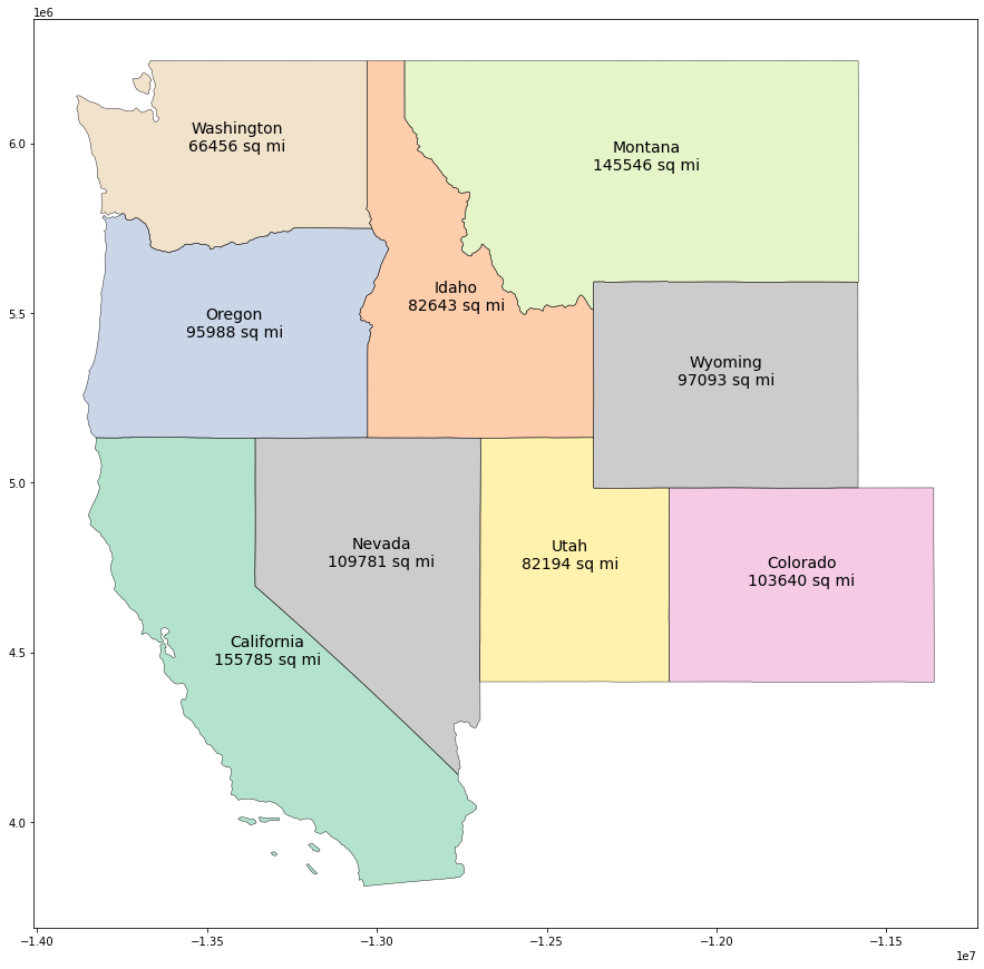
Building on the above example, we can also use a newline (\n) character to create multiline labels. This is useful if you want to display some other data column from the GeoDataFrame. Here I am plotting the state name as well as the land area of the state in square miles.
import math
fig = plt.figure(1, figsize=(25,15))
ax = fig.add_subplot()
west.apply(lambda x: ax.annotate(
    s=x.NAME + "\n" + str(math.floor(x.ALAND / 2589988.1103)) + " sq mi",
    xy=x.geometry.centroid.coords[0],
    ha='center',
    fontsize=14
),axis=1);
west.boundary.plot(ax=ax, color='Black', linewidth=.4)
west.plot(ax=ax, cmap='Pastel2', figsize=(12, 12))
!(/wp-content/uploads/2020/05/geopandas-multiline-labels-over-shapes.png)
Multiline Labels using a longitudinal offset
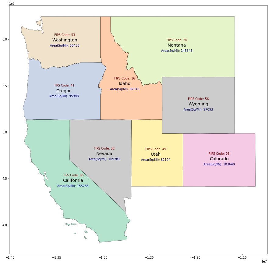
If we want to change the font size of our second data row or place the label somewhere other than directly below we will need to use a lat,long offset to draw a second label in another call to annotate()
To understand how we do this, lets first look at the data in x.geometry.centroid.coords[0]
The annotate() method requires we provide a tuple for attribute xy. In the previous apply lambda function we are passing x.geometry.centroid.coords[0].
# Get the first state
tmpdf = states.iloc[0]
# Which state
print(tmpdf.NAME)
# Get the centroid coordinates
tmpdf.geometry.centroid.coords[0]
California
(-13322855.654888818, 4465905.292663821)This is the xy coordinates of the first state. This is where our label is plotted. We can pass an offset to xy like this.
( tmpdf.geometry.centroid.coords[0][0], tmpdf.geometry.centroid.coords[0][1] - 55000 )(-13322855.654888818, 4410905.292663821)Here is the complete example where we print 3 labels. State name, land area, and FIPS code. I will also use a different font size and color for the second two labels.
import math
fig = plt.figure(1, figsize=(25,15))
ax = fig.add_subplot()
# Label 1 State Name
west.apply(lambda x: ax.annotate(s=x.NAME, xy=x.geometry.centroid.coords[0], ha='center', fontsize=14),axis=1);
# Label 2 Area using longitudinal offset
west.apply(
    lambda x: ax.annotate(
        s="Area(Sq/Mi): " + str(math.floor(x.ALAND / 2589988.1103)),
        xy= (x.geometry.centroid.coords[0][0], x.geometry.centroid.coords[0][1] - 55000 ),
        ha='center',
        color='#000077', # blue
        fontsize=10),axis=1);
# Label 3 FIPS Code using longitudinal Offset
west.apply(
    lambda x: ax.annotate(
        s="FIPS Code: " + x.STATEFP,
        xy= (x.geometry.centroid.coords[0][0] , x.geometry.centroid.coords[0][1] + 60000 ),
        ha='center',
        color='#770000', #red
        fontsize=10),axis=1);
west.boundary.plot(ax=ax, color='Black', linewidth=.4)
west.plot(ax=ax, cmap='Pastel2', figsize=(12, 12))
!(/wp-content/uploads/2020/05/geopandas-offset-labels-over-shapes.png)
Combining Overlay Maps
Here is an example where we create a larger boundary map and then overlay in a second map. It’s important to note that figsize must be specified in the first plot.
us_boundary_map = states.boundary.plot(figsize=(18, 12), color="Gray")
west.plot(ax=us_boundary_map,  color="DarkGray")
!(/wp-content/uploads/2020/05/32-geopandas-usmap-overlay-1024x593.png)
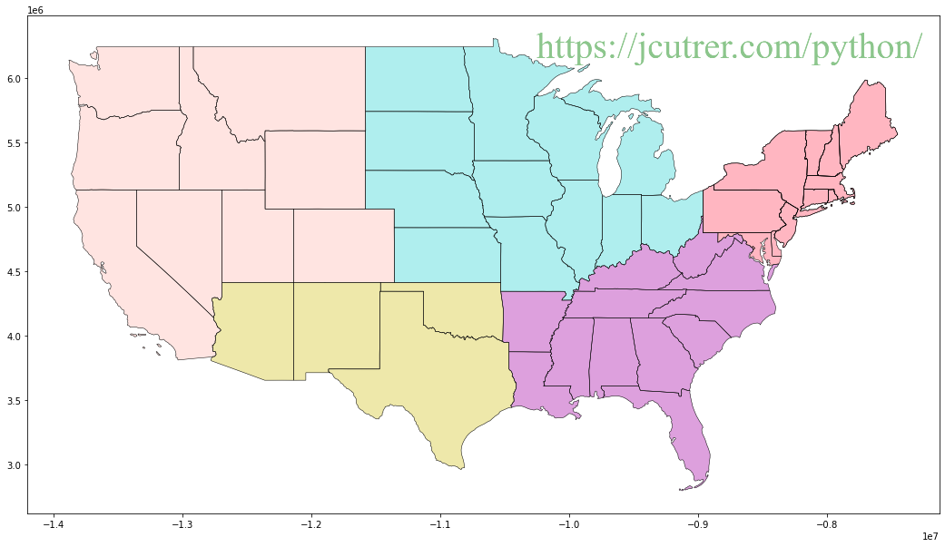
We can continue to chain our plots together to a plot of all othe United States Regions.
The first plot us_boundary_map serves as our base map.
Then we reference it with ax=us_boundary_map when we call plot() on each of our region GeoDataFrame.
west = states == 'West']
southwest = states == 'Southwest']
southeast = states == 'Southeast']
midwest = states == 'Midwest']
northeast = states == 'Northeast']
us_boundary_map = states.boundary.plot(figsize=(18, 12), color='Black', linewidth=.5)
west.plot(ax=us_boundary_map,  color="MistyRose")
southwest.plot(ax=us_boundary_map, color="PaleGoldenRod")
southeast.plot(ax=us_boundary_map, color="Plum")
midwest.plot(ax=us_boundary_map, color="PaleTurquoise")
final_map = northeast.plot(ax=us_boundary_map, color="LightPink")
!(/wp-content/uploads/2020/05/63-geopandas-us-regions-1024x593.png)
Tuning map attributes based on plot size
If you intend to plot a small map the default linewidth of 1 is probably too large. You can use decimal numbers to plot smaller lines.
tiny_map = states.boundary.plot(figsize=(5, 5), color="Black")!(/wp-content/uploads/2020/05/38-usmap-tiny.png)
tiny_map = states.boundary.plot(figsize=(5, 5), color="Black", linewidth=.25)!(/wp-content/uploads/2020/05/39-usmap-tiny-linewidth.png)
If you intend to generate a large map you should consider increasing the linewidth.
hires_map = states.boundary.plot(figsize=(50, 28), color="Gray", linewidth=4)!(/wp-content/uploads/2020/05/40-united-states-map-hires-1024x572.png)
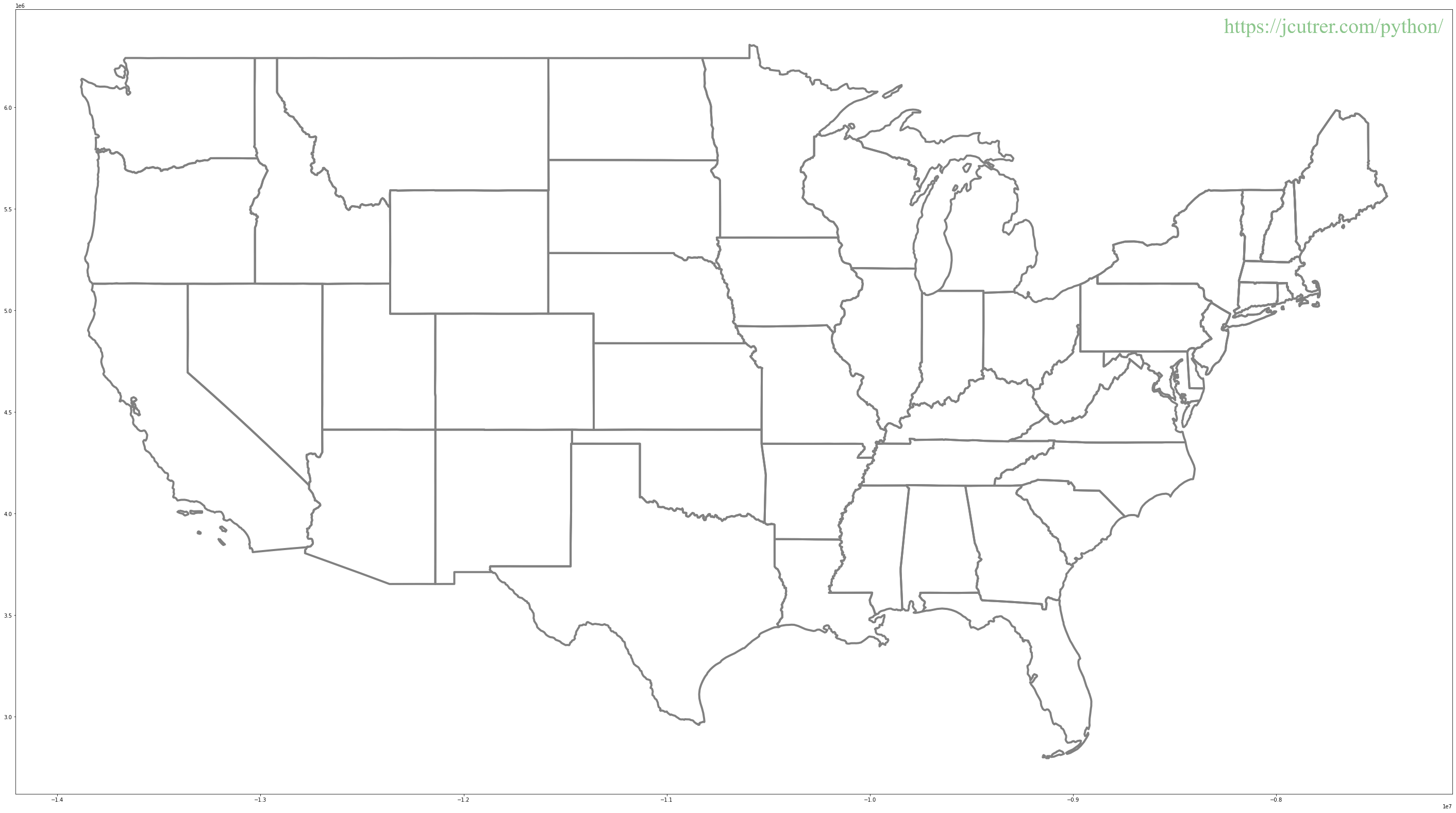
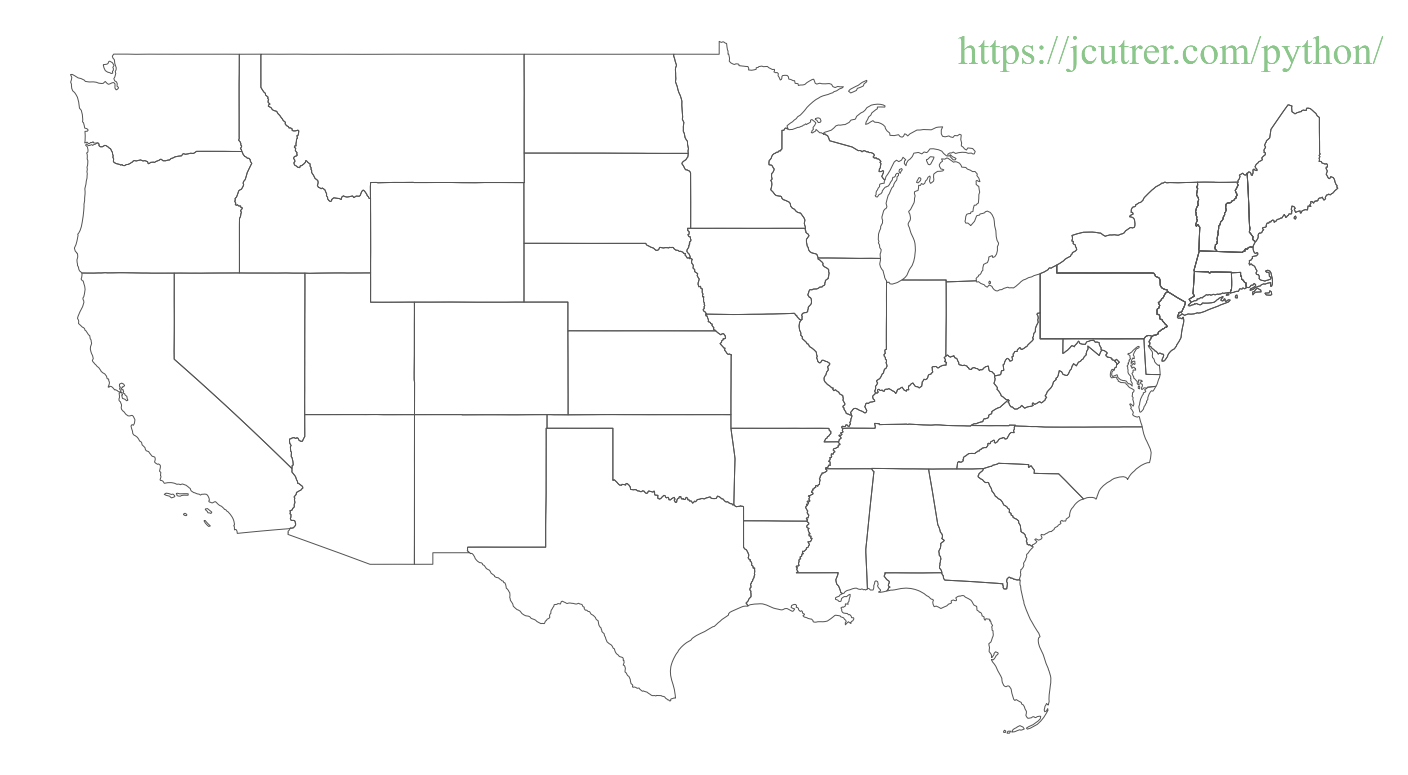
us_map = states.boundary.plot(figsize=(25, 14),  color="#555555", linewidth=1)
us_map.axis('off')
!(/wp-content/uploads/2020/05/41-united-states-map-hires-noaxis-1024x564.png)
Saving the map plot to disk
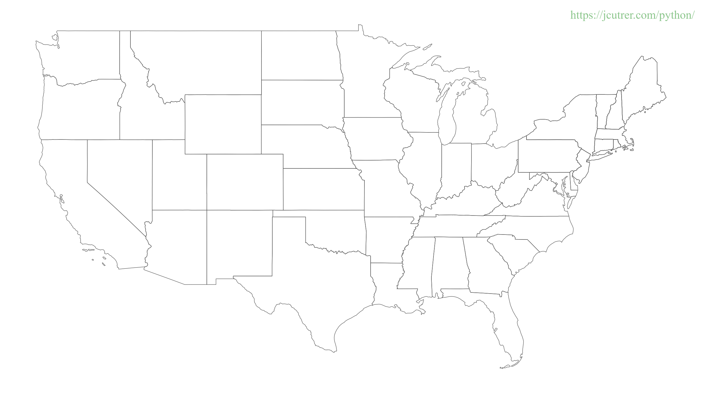
What if we want to save our map? We need to get the figure, trim whitespace and call savefig()
fig = us_map.get_figure()
fig.tight_layout()
fig.savefig('usa.png', dpi=96)
ls -al usa.png-rw-rw-r-- 1 sysadmin sysadmin 236624 May 2 03:22 usa.pngfrom IPython.display import Image
Image(filename='usa.png')!(/wp-content/uploads/2020/05/geopandas-usa-1024x573.png)
Congratulations, you are well on your way to becoming a GIS expert with geopandas. I hope this tutorial has helped you learn a little more about GeoPandas.
If this GeoPandas tutorial inspires you to create something awesome, please come back here and share it with the rest of us in the comments section below.
If you enjoyed this article you might also like (/python/learn-geopandas-plotting-tornados)
References
- (https://github.com/joncutrer/geopandas-tutorial) companion github repo- (https://geopandas.org/)- (https://en.wikipedia.org/wiki/Shapefile)- (https://lyzidiamond.com/posts/4326-vs-3857) by Lyzi Diamond- (https://matplotlib.org/tutorials/colors/colormaps.html)
(https://jcutrer.com/files/pdf/jcutrer.com-Learn-geopandas-plotting-shapefiles.pdf)
Comments are disabled (Giscus not yet configured).